In Part 1, Look Modification Transforms (LMTs) were defined as ACES-to-ACES transforms that systematically change the appearance of ACES-encoded data viewed through an ACES Output Transform.

But how do they work? What “magic stuff” happens inside that box that represents the LMT in the diagram above? And, more importantly how can one construct their own LMT?
This post will begin to step through the creation of a few LMTs at increasing levels of complexity.
[Transforms used in this article are provided as CTL code at the end of the article.]
LMT Types
LMTs can be characterized as either “empirical” or “analytic”. Empirical LMTs are derived from sampling another color reproduction process and are typically implemented as 3D LUTs that encapsulate a subsampling of such processes (Academy TB-2014-010, Section 7.2.2). Analytic LMTs are defined mathematically and are typically expressed as a set of ordered mathematical operations to adjust ACES values (Academy TB-2014-010, Section 7.2.1).
Empirical LMTs
Empirical LMTs are fairly simple to create, and can be quite powerful, but they do have limitations. ACES’ data resulting from empirical LMTs may not preserve the extended dynamic range or color gamut able to be encoded with ACES data if they are modeling an output-referred “look”.
Empirical LMT – Example 1 (match Print Film Emulation)
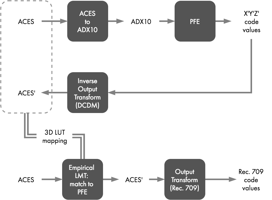
In Part 1 of this series, an empirical LMT was described that implemented a print film emulation (PFE). That PFE is in the form of a 3D-LUT that expects 10-bit log DPX as input and supplies X’Y’Z’ code values as output. Source ACES-encoded image data must be converted to a 10-bit densitometric encoding to be usable with that particular PFE LUT, and in this case, the Academy-supplied “Universal Build Transform” is used to generate ADX10 data for this purpose.
A grid of carefully selected ACES values are converted to ADX10 and then sent through the PFE 3D-LUT, resulting in X’Y’Z’ code values. Those code values are next processed through the Inverse Output Transform for DCDM (combined Inverse ODT and Inverse RRT), yielding a set of ACES’ values that encapsulate the mapping that matches the appearance of the PFE through the forward ACES Output Transform. This relationship of input to output, illustrated with the dashed gray box in Figure 2, is derived once and subsequently saved in the form of a 3D-LUT that can drop into an ACES workflow as a PFE LMT to recreate the look of that PFE.
With that PFE LMT, any ACES values processed through it should produce ACES’ values that when viewed through an Output Transform will match the appearance of the original ACES->ADX10->PFE processing chain.
Empirical LMT – Example 2 (match LUT X)
A similar process can be used to create an LMT to match any given “LUT X.”
LUT X represents a vendor-supplied rendering LUT to emulate through an ACES rendering path. LUT X expects input data encoded as “Camera X-log” in “Camera X RGB” space. LUT X outputs Rec. 709 code values.
ACES values must be transformed to the correct encoding for input to LUT X; in this case to Camera X-log with Camera X RGB primaries. This is accomplished with what is effectively the inverse of the Camera X Input Transform. (If the Input Transform linearizes a Camera X log encoding and applies a matrix from Camera X RGB to the AP0 primary set, then the inverse transform would be the exact opposite, applying a matrix to convert from AP0 to Camera X RGB followed by the Camera X log curve.)
Using an inverse Input Transform, a carefully sampled grid of ACES values is converted to the Camera X encoding needed for input to LUT X, which then produces corresponding Rec. 709 code values. Those code values can then be processed through the Inverse Output Transform for Rec. 709 (combined Inverse Rec. 709 ODT and Inverse RRT), yielding a set of ACES’ values that encapsulate a mapping that will match the appearance of LUT X through the forward ACES Output Transform. This relationship of input to output, again illustrated with a dashed gray box in Figure 3, is derived once and used to populate a 3D-LUT that can drop into an ACES workflow as an LMT to recreate the look of LUT X.
Any ACES values processed through the LUT X LMT should produce ACES’ values that when viewed through an Output Transform will match the appearance of the original ACES->Camera X encoding->LUT X processing chain.

Limitations of Empirical LMTs
Because empirical LMTs are derived from output-referred data, the range of output values from such an LMT is limited to the dynamic range and color gamut of the transform used to create the empirical LMT.
For example, consider the transform being emulated only outputs Rec. 709 at standard cinema dynamic range. If the procedure described above is used to create an empirical LMT, then any ACES input will be limited to Rec. 709 at standard cinema dynamic range at output. For the LMT to do otherwise would contradict the intention of creating an output-referred LUT.
Therefore, viewing that LMT’s output in conjunction with a P3, Rec. 2020 and/or HDR ODT (on corresponding display devices) the appearance will still match that of the Rec. 709 LUT (assuming no additional color correction is performed on the ACES’ data).
Even with additional color correction, it is also unlikely that that values outside of that limitation could be created. The ability to do so would depend both on the range of values the LMT LUT was originally made to cover (i.e. the carefully sampled grid) and how extrapolation is handled by the tool applying the LUT.
Because of these limitations, it is recommended empirical LMTs only be used when necessary to exactly match an existing look. Furthermore, empirical LMTs should certainly not be “baked in” to ACES data because that would destroy potentially useful dynamic range and color information contained in the original ACES-encoded imagery.
Fortunately, ACES’ data created with analytic LMTs can avoid this limitation because they do not use inverse Output Transforms and therefore, with careful design, will preserve dynamic range associated with the original ACES data.
Analytic LMTs will be explained in the next post.
Supporting CTL transforms
Below are download links for the CTL transforms used in the examples in this post.

